JGI Genome Portal
2008 - 2014 • JavaScript, AngularJS, Perl
The Department of Energy (DOE) Joint Genome Institute (JGI) is a national user facility with massive-scale DNA sequencing and analysis capabilities dedicated to advancing genomics for bioenergy and environmental applications. Beyond generating tens of trillions of DNA bases annually, the Institute develops and maintains data management systems and specialized analytical capabilities to manage and interpret complex genomic data sets, and to enable an expanding community of users around the world to analyze these data in different contexts over the web.

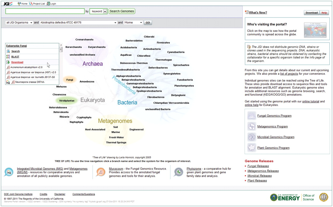
Tree of Life showing sequenced organisms and samples
The JGI Genome Portal (
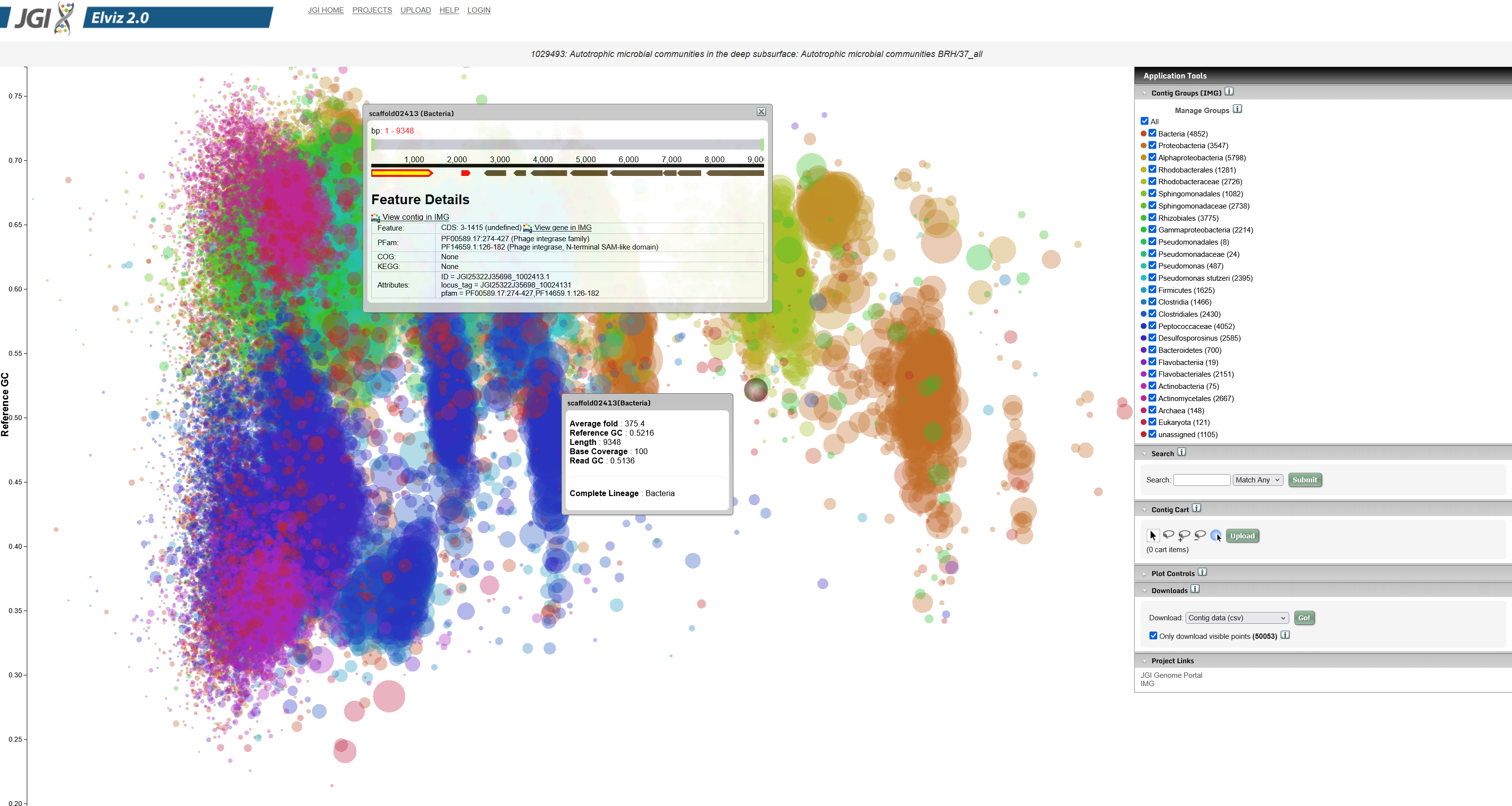
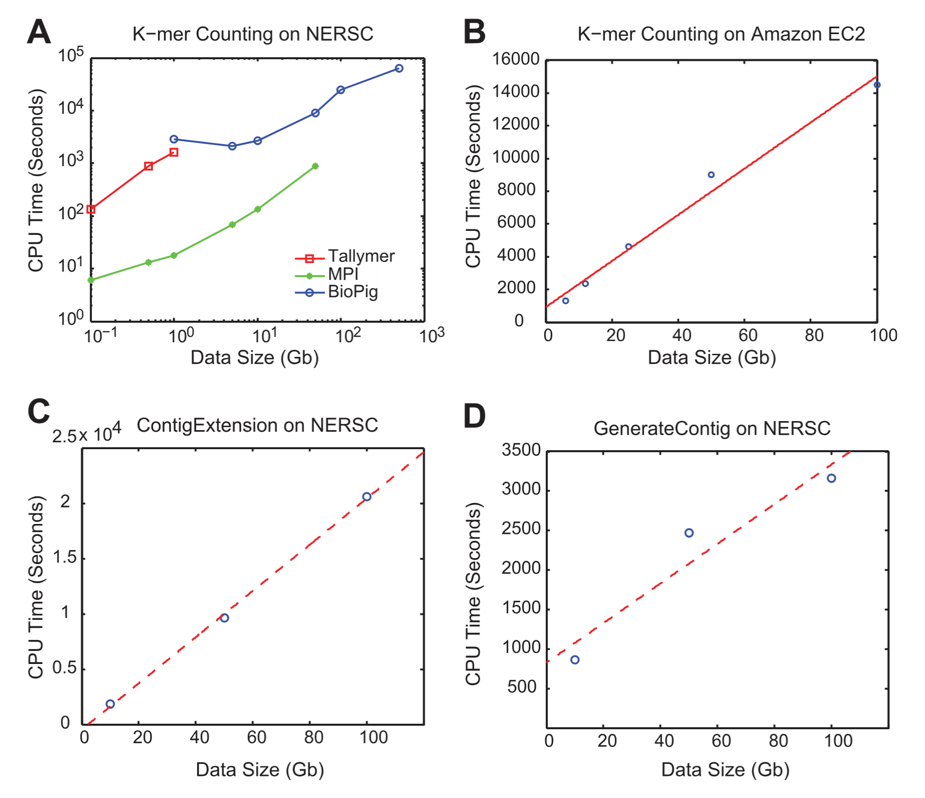
genome.jgi.doe.gov) provides a unified access point to all JGI genomic databases and analytical tools. A user can find all DOE JGI sequencing projects and their status, search for and download assemblies and annotations of sequenced genomes, and interactively explore those genomes and compare them with other sequenced microbes, fungi, plants or metagenomes using specialized systems tailored to each particular class of organisms. As Team Lead, I was responsible for this portal, which provides access to data at multiple stages of genome analysis and annotation pipelines.
We published a paper on it in Nucleic Acids Research in 2012:
The Genome Portal of the Department of Energy.
Technology
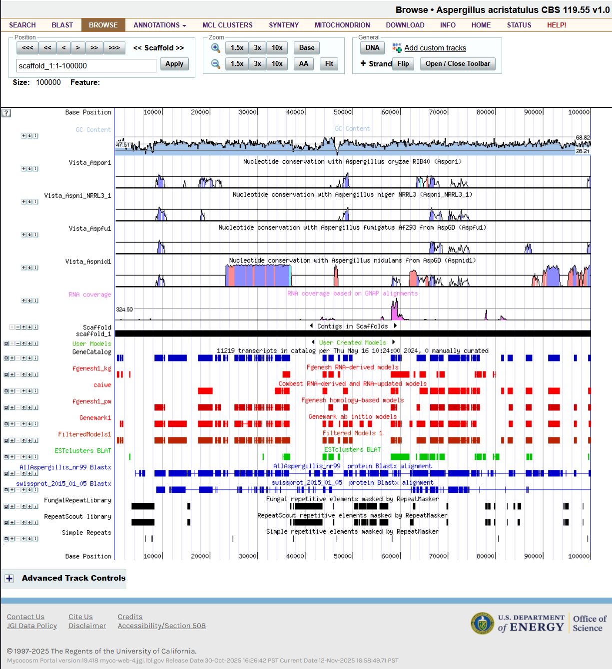
The Genome Portal is built using a combination of technologies. The genome browser (annotation and assembly viewer) is a large Perl program. When I took over, I implemented parallel rendering of the different tracks (see image below). I also added a number of long-requested features.

Genome browser implemented in Perl
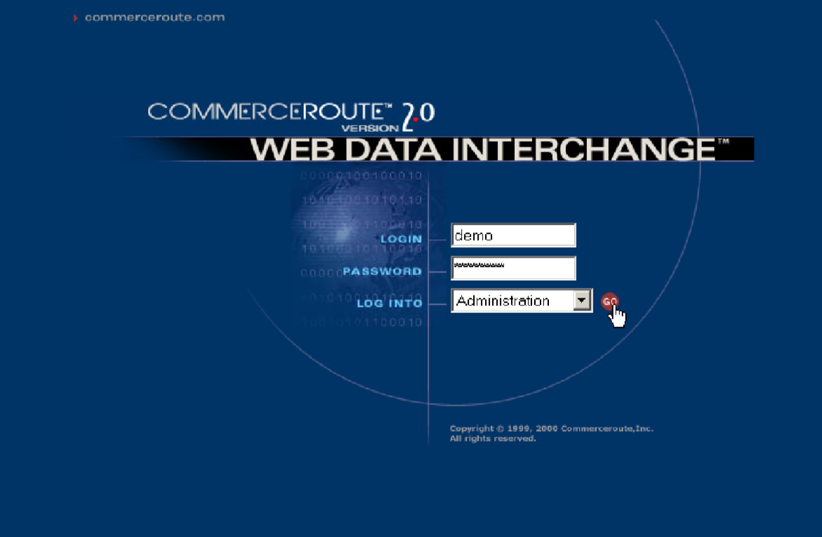
CommerceRoute Data Integration and Workflow Solutions
1997 - 2003 • C++, Microsoft MFC, Java
In 1997 I was the engineering founder of what became CommerceRoute. The first product was a workflow/Business Process Modeling (BPM) offering. It featured a client tool for defining the flow, a rules database, and a rules engine. You would define a workflow process, with tasks linked together by routes. It didn't have any restrictions on how complicated the flow could be, allowing recursive flows and multiple instances of the same task. Right away people wanted to pull in data from external sources, and use them in the logic. We started adding connections to databases, LDAP, SAP, FTP, local files, and formats like XML, EDI, flat files, etc. With time people started to use the flows for data movement instead of just process automation. That's how the next product was born.
Data Integration
Building upon the powerful engine, we developed the CommerceRoute data integration solution, which handles transformations and transfers between sources and targets, and implemented the RosettaNet B2B framework. The complete solution was later sold as the Syncx integration appliance, reducing support costs.
CommerceRoute SaaS
The launch of CommerceRoute Syncx was accompanied by a new SaaS offering: commerceroute.net All Syncx appliances talked to commerceroute.net and reported health and usage data. As needed, updates were pushed to the appliances. This included both OS level security updates and new features.

CommerceRoute SaaS web interface
Acquisition
In 2003 a new company was formed to acquire the product. The new company was called Jitterbit, and it acquired the technology from CommerceRoute. A few of the founders of CommerceRoute stayed on to start Jitterbit. Jitterbit is now a cloud-based data integration company recognized as a leader and visionary in the iPaaS field.
Technology and Architecture
The engine was written in C++ using boost libraries. The workflow client was written in C++ using Microsoft's MFC library. For a while Jitterbit open sourced the product, and it is
available on SourceForge. After a while Jitterbit completely stopped using the workflow product and focused on the data integration product. But it wasn't until 2009 that they pushed an update to remove the workflow logic from the code. So you can still find my original code in the repository by
going back through the history. For example the
RoutingEngineCore.cpp file handles the routing logic for the workflow.
Scaling
The workflow engine is multi-threaded and will detect the number of cores available and use them. It is also able to scale as a cluster of machines. In this mode, synchronization is handled via the database. The standard Syncx appliance configuration started with 2 multi-core machines and one database server. From there, customers would add capacity as needed by adding more machines. This was designed to be a simple process and was done via the web interface. For enterprises, they would add a second database server, which would run in a two-phase commit mode to ensure data consistency. In that mode, each query is executed in a way that the transaction succeeds only after both database servers have confirmed a successful commit. During one demo we did to a large enterprise customer, we used a workflow with complex logic with loops and data dependencies between tasks. In the middle of the demo, we pulled the power to the machine and waited for it to restart. When it came back online, the process continued and completed successfully. This was possible because the source of truth for the workflow logic and state was always the database.
Multi-dimensional Clustering Algorithm
1997 - 1999 • C++, Java
When I joined the Scientific Data Management R&D group at Lawrence Berkeley Laboratory in 1997, the first project I worked on was a multi-dimensional clustering algorithm. As the high energy physics community was preparing for the Large Hadron Collider, they looked to our group to help manage the data. My task was to come up with an algorithm to find clusters of collision events. An "event" is when two particles collide in a collider. The data describes how many of each type of elementary particle were produced in the collision, along with data for each particle, such as momentum and energy.
The Curse of Dimensionality
We were dealing with 100 - 150 columns or dimensions of data. Classical clustering algorithms like k-means or hierarchical clustering break down when you have that many dimensions. This is known as the curse of dimensionality. The events tend to cluster into groups of events that are similar. My task was to find them.
Algorithm
I relied on the fact that the data is very sparse in higher dimensions. Since the number of events was large but known, I decided to use a hash table to store information about only the non-empty cells. The algorithm was:
- Read the data (one pass) and populate the cells
- Sort the cells by the number of events
- Grow a cluster around the largest cell. Find all neighbors of Manhattan distance 1. Stop growing when events in a cell are below a threshold, or when the gradient increases.
- Then grow the cluster around the next available largest cell.
- Repeat until all cells are in a cluster
Technology
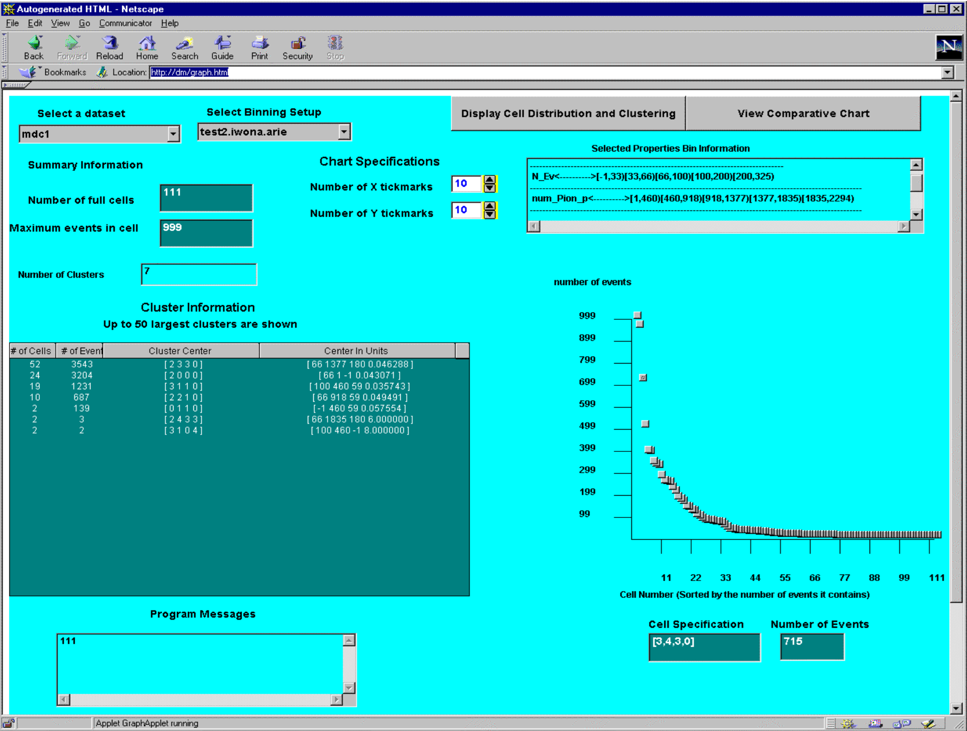
The algorithm was implemented in C++ on Solaris. I used a hash table to store the data. In addition to the algorithm, we also developed a Java Applet that could be used to explore the clusters.

Java applet for exploring multi-dimensional clusters
Selecting the bins was a task of its own. The Java Applet allowed you to explore what bins yielded the best clusters.
Compressed Bitmap Index
1997 - 1999 • C++
To be able to serve high energy physics data from tape systems, we needed to be able to quickly estimate the size of a result set for a particular query before the data retrieval request was executed. This would allow the scientists to refine their queries before retrieving the data. To this end, I researched and implemented a specialized compressed bitmap (a.k.a. bit-sliced) index that is highly effective for range queries. The queries were logical joins of ranges on several columns. A key feature of this work is the ability to perform query execution directly without needing to decompress the index first. One idea was to run clustering on the data, and re-order the events based on clusters. In 1995 Gennady Antoshenkov developed the Byte-aligned Bitmap Code (BBC), a well-known scheme for bitmap compression. Our work is similar, but we added several novel features to make them more efficient for our use case.
Algorithm
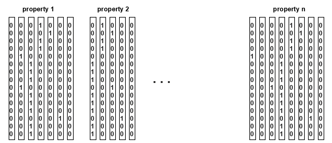
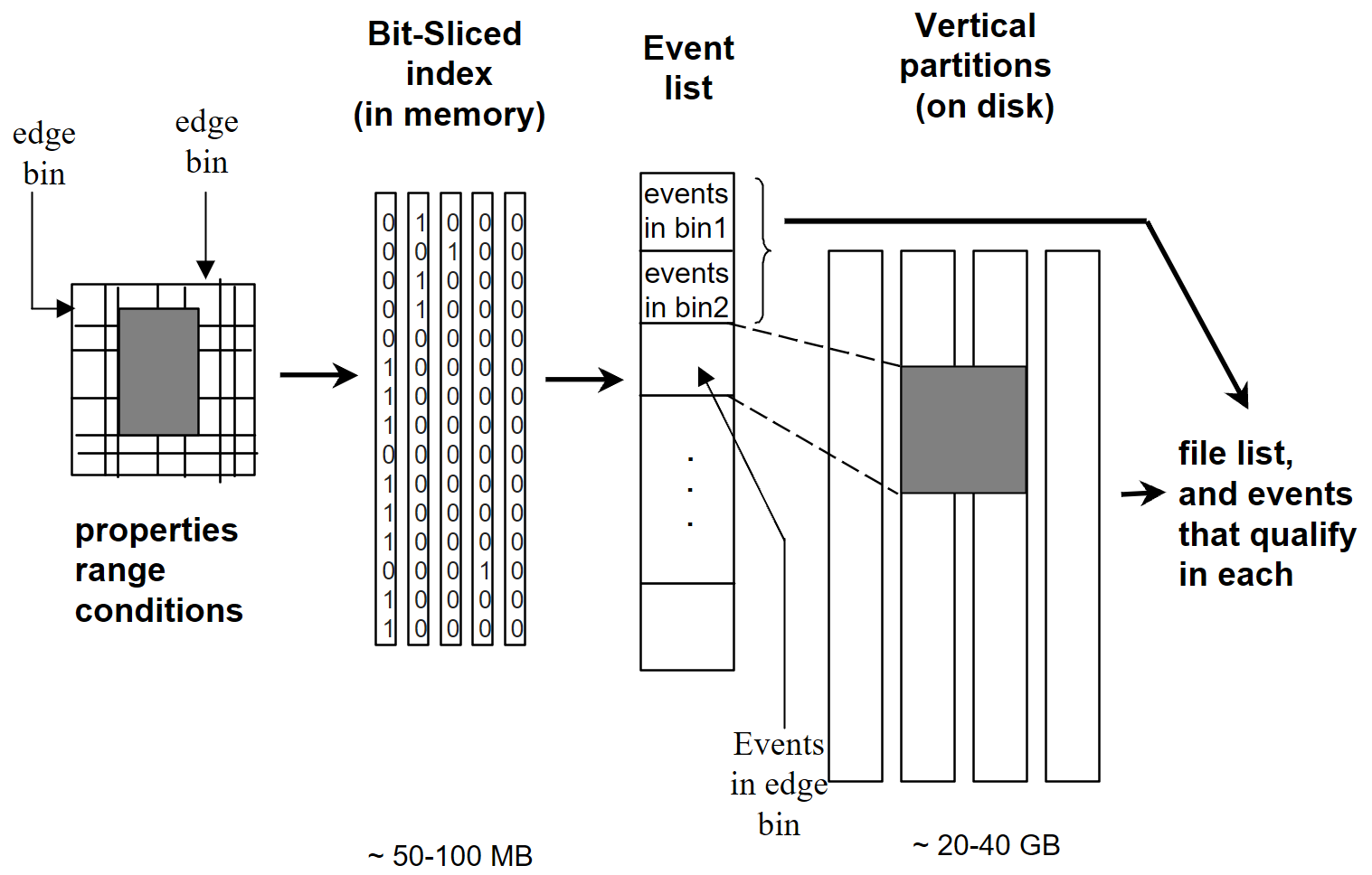
We assume that the objects are stored in a certain order in the index, and this order does not change. Thus, we first generate vertical partitions for each of the 100 properties. If all the properties are short integers, the size of all the partitions is 20 GBs (100 × 2 × 10⁸ bytes). The size doubles if all were real numbers. The vertical partitions are stored on disk. Now the bit-sliced index is designed to be a concise representation of these partitions, so that it is much smaller and can be stored in memory. Since the properties we deal with are numeric, we can partition each dimension into bins. For example, we can partition the "energy" dimension into 1–2 GeV, 2–3 GeV, and so on. We then assign to each bin a bit vector, where a "0" means that the value for that object does not fall in that bin, and "1" means it does.

Example of bit-sliced index partitions
The figure shows an example where Property 1 was partitioned into 7 bins, Property 2 into 5 bins, etc. Note that only a single "1" can exist for each row of each property, since the value only falls into a single bin.
We now compress the vertical bit-vectors using a modified version of run-length encoding. The advantage of this scheme is that boolean operations can be performed directly on the compressed vectors without decompression. This scheme is particularly effective for highly skewed data such as High Energy Physics data. Our version of run-length encoding does not encode short sequences into counts. Instead, it represents them as-is. A single bit in each word indicates whether it is a count or a pattern. Results show a compression factor of 10-100. The choice of bins and bin boundaries has a significant impact on compression. Assume 100 properties, each with 10 bins. This requires 10¹¹ bits before compression. With a compression factor of 100, the space required is 10⁹ bits, or about 125 MBs. This can be stored permanently in memory. Note that it is not necessary to keep all bit slices in memory. Only the most relevant slices for a query need to be retained.
Logical Operations on Bit-Slices
The compression scheme described above permits logical operations on the compressed bit-slices (bitmap columns). This is an important feature of the compression algorithm used, since it makes it possible to do the operations in memory. These operations take as input two compressed slices and produce one compressed slice (the input for "negation" is only one bit-slice). All logical operations are implemented the same way:
- The state ["0" or "1"] at the current position and the number of bits of the current run (number of consecutive bits of that same state), 'num', from each bit-slice, are extracted (decoded).
- The result is created (encoded) by performing the required logical operation (AND, OR, XOR) on the state bits from each bit-slice and subtracting the smaller 'num' from the larger and appending the result to the resulting bit-slice. The resulting bit-slice is encoded as we go along, using the most efficient method for the size of its run lengths.
An example: pseudo code for logical or:
function bmp_or( bitslice left,
                 bitslice right )
{
  while( there_are_more_bits(left)
    and there_are_more_bits(right) )
  {
    lbit = decode( left, lnum );
    rbit = decode( right, rnum );
    result_bit = lbit | rbit;
    result_num = min( lnum, rnum );

    lnum = lnum - result_num;
    rnum = rnum - result_num;
    encode( result,
            result_bit,
            result_num );
  }
  return result;
}
Cosmic Microwave Background (CMB) Spectrum Analysis
1996 - 1998 • Fortran
This research involved a detailed analysis of observations related to the Cosmic Microwave Background (CMB) radiation intensity, a relic of the Big Bang. In 1995 and 1996 I worked on the Isotope Explorer (see below) while also completing MSc in Physics, taking classes at UC Berkeley. When it came time to write my thesis, Dr. Richard Firestone of the Isotopes Project at LBL put me in touch with Dr. George Smoot, who had recently gathered data from his DMR experiment onboard the COBE satellite.
Nobel Prize
The DMR data showed that the CMB was not uniform, but had a large difference in one direction, and small variations all around. This dipole pattern showed the motion of our solar system, and our local group of galaxies relative to the CMB. George received the Nobel Prize in Physics in 2006 for this work.

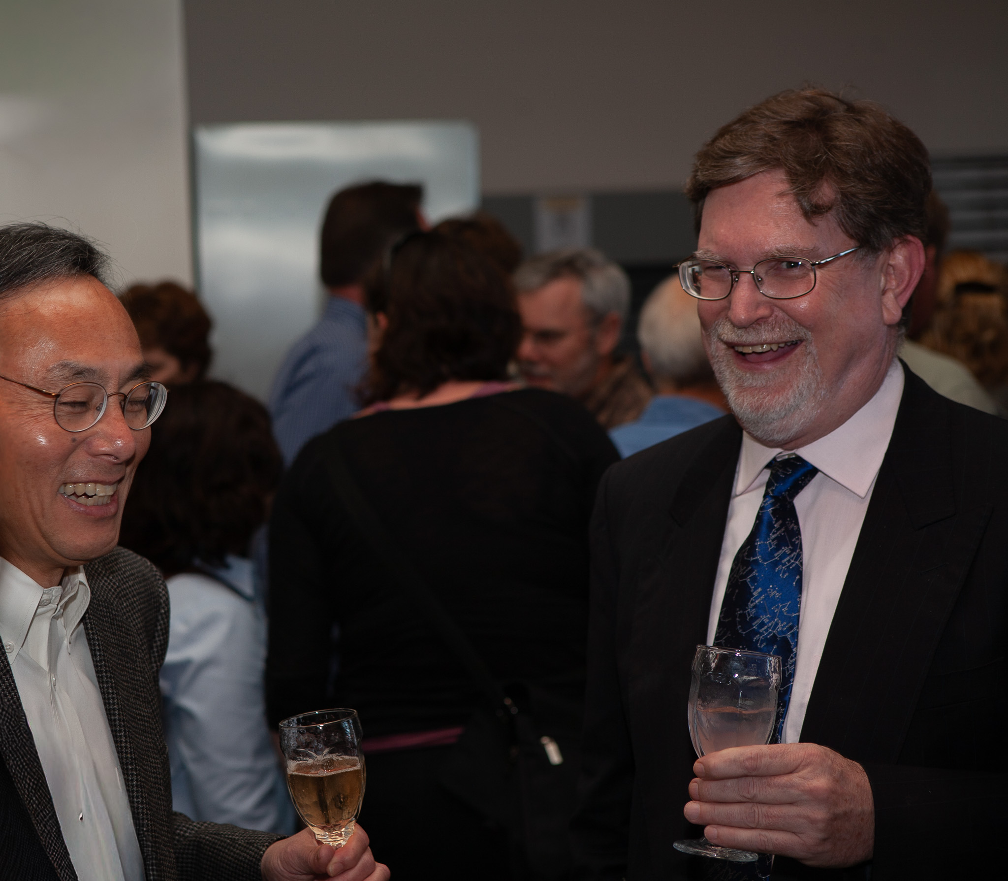
Dr. Chu and Dr. Smoot on the day of the Nobel Prize announcement. Photo: Henrik Nordberg
The image shows Dr. George Smoot and Dr. Steven Chu, who was the lab director at the time and also the Secretary of Energy, on the day of the announcement of the Nobel Prize in Physics in October 2006. Dr. Chu received the Nobel Prize in Physics in 1997. As a side note, Berkeley Lab is an amazing place. George would tell me stories about his advisor, Luis Alvarez, who also was a Nobel Laureate in Physics (1968). So you know, I still have a few years... :) I would attend the INPA (Institute for Nuclear and Particle Astrophysics) seminars on a regular basis. Whenever a new important paper in physics was published, the authors would come and give a talk. The lab has had 17 Nobel Prize winners affiliated with it.
Data Analysis
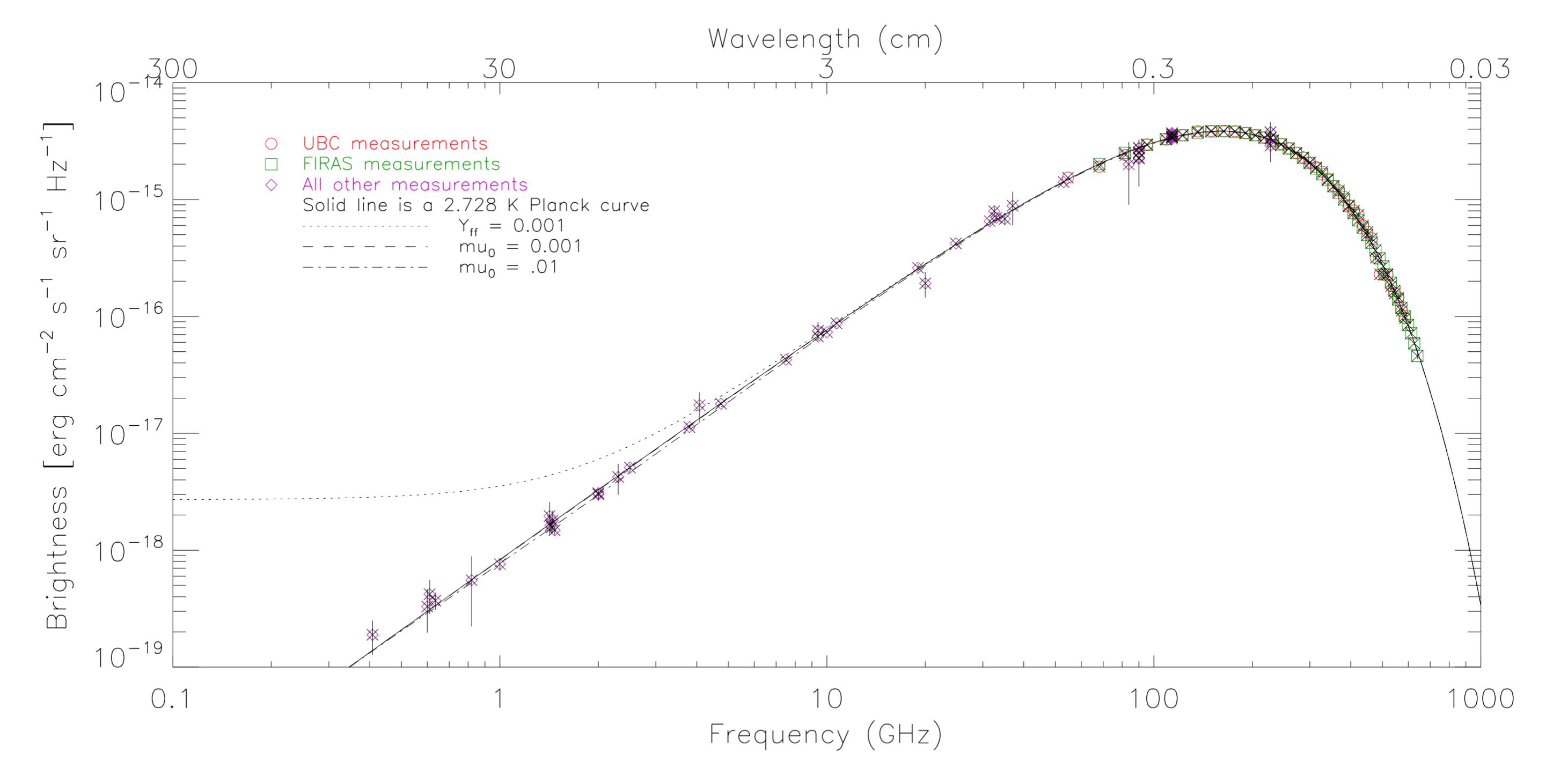
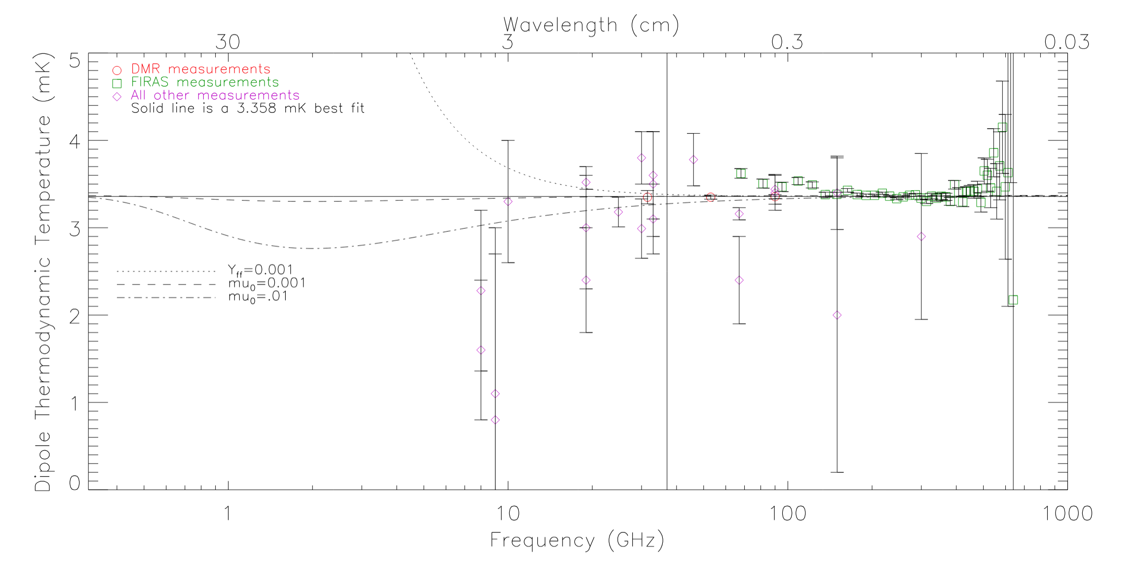
In addition to the COBE data, George and I collected all known published data on the CMB spectrum. I then wrote Fortran code to fit the data to various models.

Brightness as a function of frequency of the CMB

Thermodynamic temperature as a function of frequency of the CMB dipole
Levenberg-Marquardt Method
I first tried gradient descent to fit the data to a model. It didn't converge in a reasonable time.
The Levenberg-Marquardt method is used to iterate to the optimal $\chi^2$.
It combines the Steepest Decent and Grid Search methods into an
algorithm with a fast convergence.
By Taylor expansion of $\chi^2$ we have
$$\begin{multline*}\chi^2 = \chi^2(0)+\sum_i \frac{\partial \chi^2}{\partial x_i}x_i\\+\frac{1}{2}\sum_{i,j}\frac{\partial^2\chi^2}{\partial x_i\partial x_j}x_ix_j+...\end{multline*}$$
which we can write as
$$\chi^2\approx \gamma - \vec{d}\cdot\vec{a}+{1\over 2}\vec{a}^T\cdot{\bf D}\cdot\vec{a} \tag{1}\label{eq:parabola}$$
where $\vec{d}$ is a vector and ${\bf D}$ is a square matrix.
This leads to
$$a_{\rm min}\approx a_{\rm cur}+{\bf D}^{-1}\cdot\left[-\nabla \chi^2(a_{\rm cur})\right] \tag{2}\label{eq:just_above}$$
We measure $x_i$ and $s_i$. Our fitting function is $t(\vec{a})$.
$$\chi ^2 = \sum_{q,r}{\left\{ (s-t(\vec{a}))_q
{\bf M}_{qr}^{-1} (s-t(\vec{a}))_r \right\}}$$
$${\partial \chi ^2 \over \partial a_i} = -2\sum_{q,r}{\left\{
\left({\partial t(\vec{a}) \over \partial a_i}\right)_q
{\bf M}_{qr}^{-1} (s-t(\vec{a}))_r \right\}}$$
$$\begin{multline*}{\partial ^2 \chi ^2 \over \partial a_i \partial a_j} = 2\sum_{q,r}\left[
\left\{\left({\partial t(\vec{a}) \over \partial a_i}\right)_q
{\bf M}_{qr}^{-1} \left({\partial t(\vec{a}) \over \partial a_j}\right)_r \right\}-
\right.\\ \left.
\left\{\left({\partial^2 t(\vec{a}) \over \partial a_i\partial a_j}\right)_q
{\bf M}_{qr}^{-1} (s-t(\vec{a}))_r \right\}
\right]\end{multline*}$$
Define
$$\beta_i\equiv -{1\over 2}{\partial \chi^2 \over \partial a_i}$$
and
$$\alpha_{ij}\equiv {1\over 2}{\partial^2\chi^2 \over \partial a_i\partial a_j}$$
We approximate $\alpha$ with [Press, W.H., et al. Numerical Recipes]
$$\alpha_{ij}\approx\sum_{q,r}\left\{
\left({\partial t(\vec{a}) \over \partial a_i}\right)_q
{\bf M}_{qr}^{-1} \left({\partial t(\vec{a}) \over \partial a_j}\right)_r
\right\}$$
Following equation (\ref{eq:parabola}) we have ${\bf\alpha}={1\over 2}
{\bf D}$ and we can re-write eq.~(\ref{eq:just_above}) as
$$\sum_i \alpha_{ij}\delta a_i=\beta_j$$
Let
$$\delta a_i={1\over \lambda \alpha_{ii}}\beta_i,$$
where $\lambda$ is a small positive constant and
$$\begin{aligned}
\alpha_{ii}' &\equiv \alpha_{ii}(1+\lambda) \\
\alpha_{ij}' &\equiv \alpha_{ij}\;\;\;\;\;(i\neq j)
\end{aligned}$$
$$\sum_i \alpha_{ij}'\delta a_i=\beta_j \tag{3}\label{eq:numrec14.4.14}$$
The idea of the Levenberg-Marquardt method is summarized in the following procedure
- Compute $\chi^2(\vec{a})$.
- $\lambda \leftarrow 0.001$.
- Solve the linear equations (\ref{eq:numrec14.4.14}) for $\delta\vec{a}$
and evaluate $\chi^2(\vec{a}+\delta\vec{a})$.
- If $\chi^2(\vec{a}+\delta\vec{a})$ is smaller than a certain threshold,
then stop.
- If $\chi^2(\vec{a}+\delta\vec{a})\geq\chi^2(\vec{a})$, increase
$\lambda$ by a factor 10. Go to Step 3.
- If $\chi^2(\vec{a}+\delta\vec{a})<\chi^2(\vec{a})$, decrease
$\lambda$ by a factor 10. Go to Step 3.
We also need to calculate the standard deviations, $\delta a_i$,
$${\bf C}={\bf{\alpha}}^{-1}$$
and thus,
$$\delta a_i = \sqrt{\Delta \chi _\nu ^2}\sqrt{C_{ii}},$$
where $\Delta \chi _\nu ^2$ is a change in $\chi ^2$ per degree of
freedom corresponding to a change in one of the parameters $a_i$.
The Levenberg-Marquardt method was applied to the CMB datasets with great success.
The method has several times more rapid convergence than the Steepest Descent
and Grid Search methods. The latter two were tried first, but neither had reasonable
convergence times, as they were implemented.
Summary
This work shows strong evidence for the hot Big Bang model. The monopole CMB spectrum is very close to a blackbody spectrum. There is a lot more math and physics than I can fit here. I wrote my
Master's thesis on this, and Dr. Smoot and I wrote a paper with a
more extensive analysis of the data. Probably the most fun result is how we put an upper bound on the tachyon coupling constant, and an upper bound on the mass of a second species of photon.
Sadly George passed away in 2025.
Query Estimator for Petabyte Storage Systems
1998 - 1999 • C++
Retrieving large subsets of data from tape-based datasets is very expensive both in terms of computer and system resources, as well as the total elapsed time for a query to be completed. Therefore, it is quite useful to provide an estimate of the amount of data and the number of files that need to be retrieved for a potential query. Often, users start a query, get frustrated with the length of time to perform the analysis, and abort the query. An important optimization strategy is to prevent such non-productive activities by providing a quick estimate of the size of the returned data, and a time estimate of how long it will take to retrieve the data. I designed and developed such a "query estimator" by taking advantage of the compressed bitmap index used to evaluate a query.

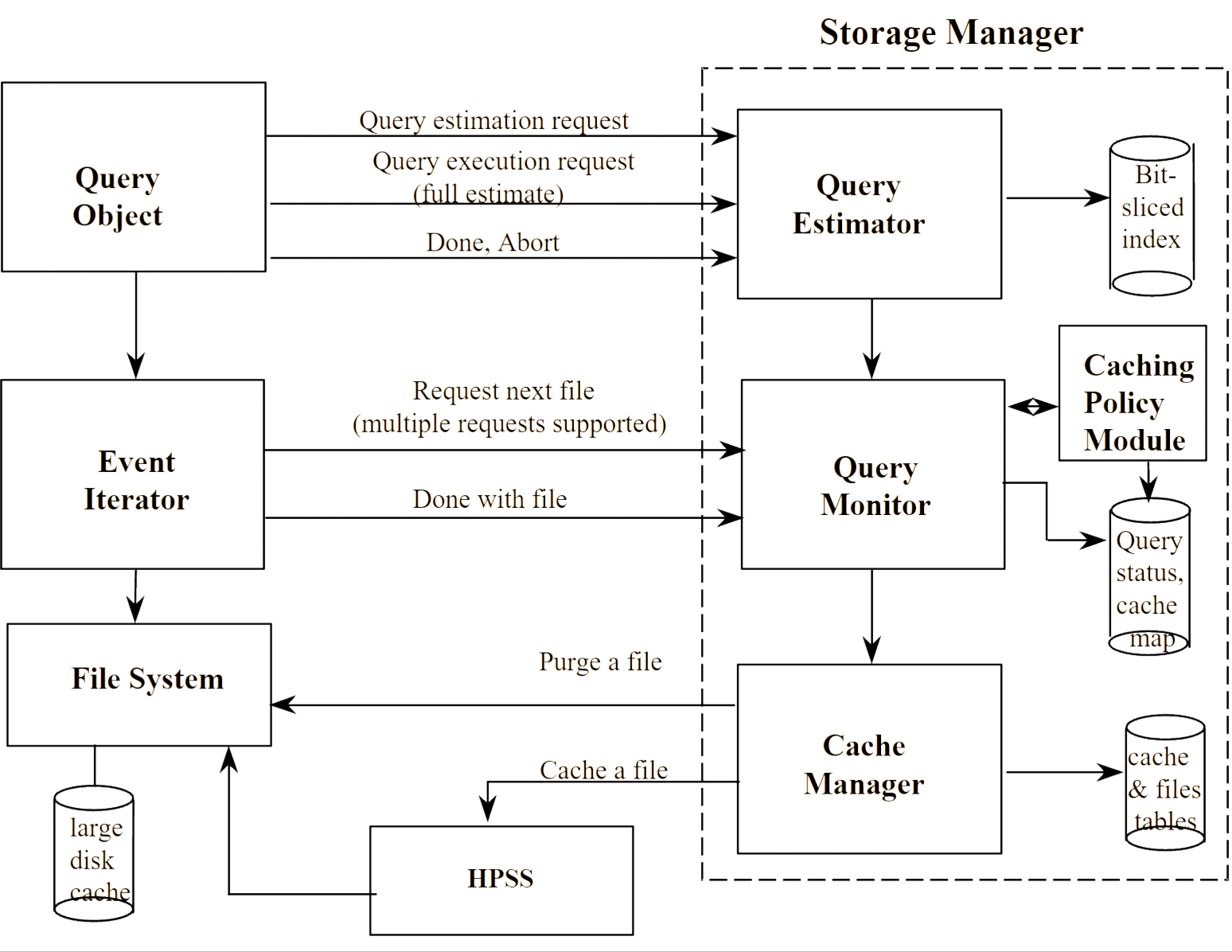
Query Estimator
Technology

Storage Manager
The query estimator was written in C++ and boost libraries, running on Solaris and Linux. It talked to other components in the distributed system via CORBA.
Automated Testing for Epic EMR workflows
2024 - 2025 • JavaScript • Playwright
Epic is an Electronic Medical Record (EMR) system used by hospitals to manage patient data, and run hospital operations. Think scheduling, billing, and patient care. It's a large system, made even more complex by the fact that hospitals usually configure it to their own needs, creating a set of workflows. Epic is now on a quarterly release cycle, and incentivises hospitals to stay up to date with the latest version. Behind the scenes, there is a lot of testing going on for every release. We designed and built a system where this testing could be automated.
How it works
The test steps were already managed by ALM (formerly HP ALM, now managed by Opentext). In ALM you have the test descriptions, instances, outcomes, and defects. Using a small VBScript we were able to add a button to the ALM UI that kicked off a test or set of tests by calling a GitHub API that runs a GitHub Actions workflow. We passed in the test ID to the workflow, and it ran a JavaScript program that retrieved the test details from ALM, and then located and executed the matching Playwright script. When the script finished, it created a test run in ALM and attached the results. If it failed, it would also create an ALM defect and attach a screenshot of the failure and a video of the run (if so configured). It would also email the screenshot, video, and failure message to the user that kicked off the test. For troubleshooting purposes, the emails contain a secret link that takes you to the GitHub run. Useful if something unexpected happened.
Workflow Diagram
flowchart TD
USER(["👤 User"])
BUTTON["Click 'Run Test' Button<br/>in ALM UI"]
VBSCRIPT["VBScript executes"]
API["Call GitHub API<br/>with Test ID"]
ACTIONS["GitHub Actions<br/>Workflow Starts"]
JAVASCRIPT["JavaScript Program Runs"]
FETCH["Retrieve Test Details<br/>from ALM"]
LOCATE["Locate Matching<br/>Playwright Script"]
PLAYWRIGHT["Execute Playwright Script"]
EPIC[("Epic EMR<br/>Test Environment")]
DONE["Test Completes"]
PASSED{Passed?}
TESTRUN["Create Test Run in ALM<br/>Attach Results"]
DEFECT["Create Defect in ALM"]
ATTACH["Attach Screenshot 📸<br/>Attach Video 🎬"]
EMAIL["📧 Send Email Notification<br/>Include link to GitHub run"]
USER --> BUTTON
BUTTON --> VBSCRIPT
VBSCRIPT --> API
API --> ACTIONS
ACTIONS --> JAVASCRIPT
JAVASCRIPT --> FETCH
FETCH --> LOCATE
LOCATE --> PLAYWRIGHT
PLAYWRIGHT <--> EPIC
PLAYWRIGHT --> DONE
DONE --> PASSED
PASSED -->|"✅ Yes"| TESTRUN
PASSED -->|"❌ No"| DEFECT
DEFECT --> ATTACH
TESTRUN --> EMAIL
ATTACH --> EMAIL
EMAIL --> USER
style USER fill:#6366f1,stroke:#818cf8,stroke-width:2px,color:#fff
style BUTTON fill:#1e3a5f,stroke:#4a90d9,stroke-width:2px,color:#fff
style VBSCRIPT fill:#1e3a5f,stroke:#4a90d9,stroke-width:2px,color:#fff
style API fill:#24292e,stroke:#6e7681,stroke-width:2px,color:#fff
style ACTIONS fill:#24292e,stroke:#6e7681,stroke-width:2px,color:#fff
style JAVASCRIPT fill:#24292e,stroke:#6e7681,stroke-width:2px,color:#fff
style FETCH fill:#1e3a5f,stroke:#4a90d9,stroke-width:2px,color:#fff
style LOCATE fill:#2d4a3e,stroke:#45b26b,stroke-width:2px,color:#fff
style PLAYWRIGHT fill:#2d4a3e,stroke:#45b26b,stroke-width:2px,color:#fff
style EPIC fill:#7c3aed,stroke:#a78bfa,stroke-width:2px,color:#fff
style DONE fill:#374151,stroke:#6b7280,stroke-width:2px,color:#fff
style PASSED fill:#1f2937,stroke:#9ca3af,stroke-width:2px,color:#fff
style TESTRUN fill:#065f46,stroke:#34d399,stroke-width:2px,color:#fff
style DEFECT fill:#7f1d1d,stroke:#f87171,stroke-width:2px,color:#fff
style ATTACH fill:#7f1d1d,stroke:#f87171,stroke-width:2px,color:#fff
style EMAIL fill:#d97706,stroke:#fbbf24,stroke-width:2px,color:#fff
Payment Gateway
2023 • TypeScript • Express.js
John Muir Health needed a way to handle payments for both accepting donations to their foundation and accepting payments on invoices in the internal Workday system. Since we wanted to avoid handling credit cards and all the PCI regulations that come with that, we decided to implement a payment gateway. We selected JP Morgan Chase's payment tech offering.
How it works
There are two entrypoints:
- Donations from the website
- Invoices from Workday
For donations, we have a form on the website that collects information about the donor, which gets posted to the payment gateway API. For Workday, we configured it to call the payment gateway API with the invoice information. The API then redirects the browser to the Chase API and provides a simple form with a known string that Chase replaces with the actual credit card form fields. The user fills in the payment details, while still being on the Chase domain, and when they click submit Chase attempts to charge the payment and then redirects back to our API and we can render a result based on whether the payment succeeded. It's a simple way of completely offloading the sensitive payment details to a payment provider.
Isotope Explorer
1995 • C++, Borland OWL, Microsoft MFC
In 1995 I moved from Sweden to Berkeley to work on a visualization tool for nuclei of isotopes at Lawrence Berkeley Laboratory. Originally called VuENSDF, it is a tool for exploring the nuclear data from the ENSDF database. Up till then, when you needed to access nuclear energy level data, you used the Table of Isotopes (ToI), which was a thick book. ToI was published by the Isotopes Project, a research group at the Nuclear Science Division of LBL. That group was headed by Nobel Laureate Glenn T. Seaborg, who still checked in on us from time to time. Dr. Seaborg was famous for the discovery of the elements plutonium, americium, curium, berkelium, californium, einsteinium, fermium, mendelevium, nobelium, and seaborgium.

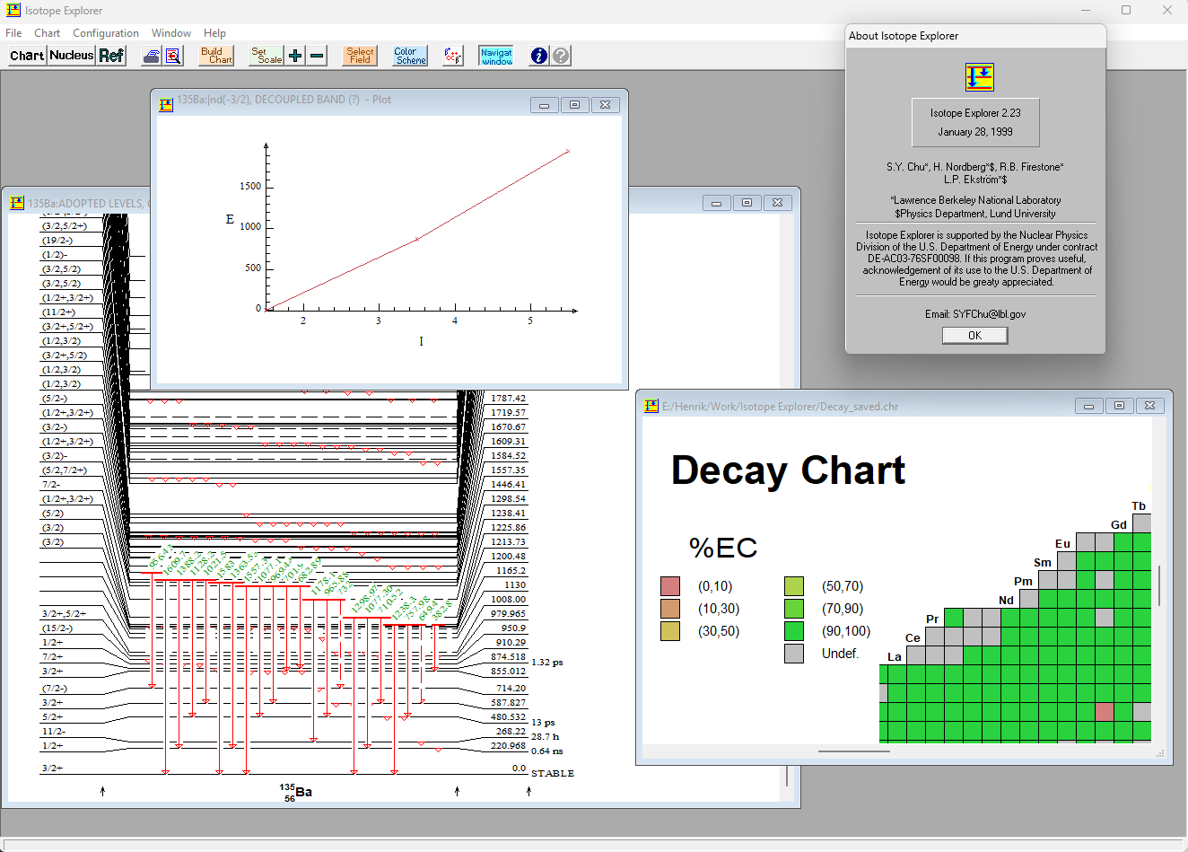
Isotope Explorer visualization tool
Technology
The tool was written in C++ and Borland's OWL library for Windows. One weekend I was reading the C code for the Unix Telnet server and decided to see if I could talk to it from Isotope Explorer. This led to us adding access to a large document set of references to the nuclear data. This was a web service before the term was invented.
Features
Isotope Explorer can display level drawings, coincidences, tables, band plots, nuclear charts, chart data and literature references.
BatMUD
1991 • LPC
A MUD (Multi-User Dungeon) is an online role-playing game. In 1991 I was at the university and joined
BatMUD as a player. Back then you accessed the game via a telnet client. I wizzed (reached level 20 and beat Tiamat) and started extending the game as all wizards do. This is how I discovered my love of programming. I started working on the backend, adding a 'feelings' system and the first global event (orch raids), among other things. The coding for LPC MUDs is in LPC, an object-oriented version of C. My player character is the Archwizard Plura.
Browser extension: Copy That
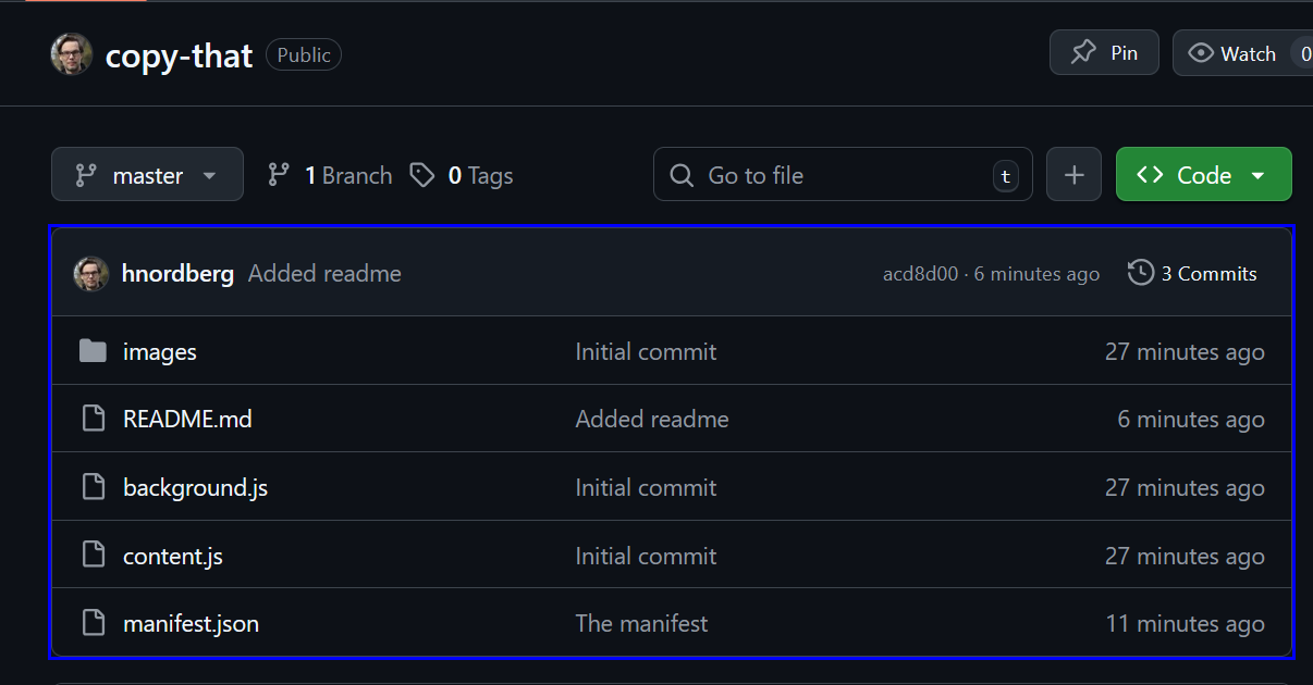
Copy-That is a browser extension that allows you to copy text or HTML from an element on the page to the clipboard. It now supports math equations so you can copy them from the web and paste into Microsoft applications (Word, PowerPoint, etc.) and have them rendered correctly.
Photo Stats: A Python EXIF scanner
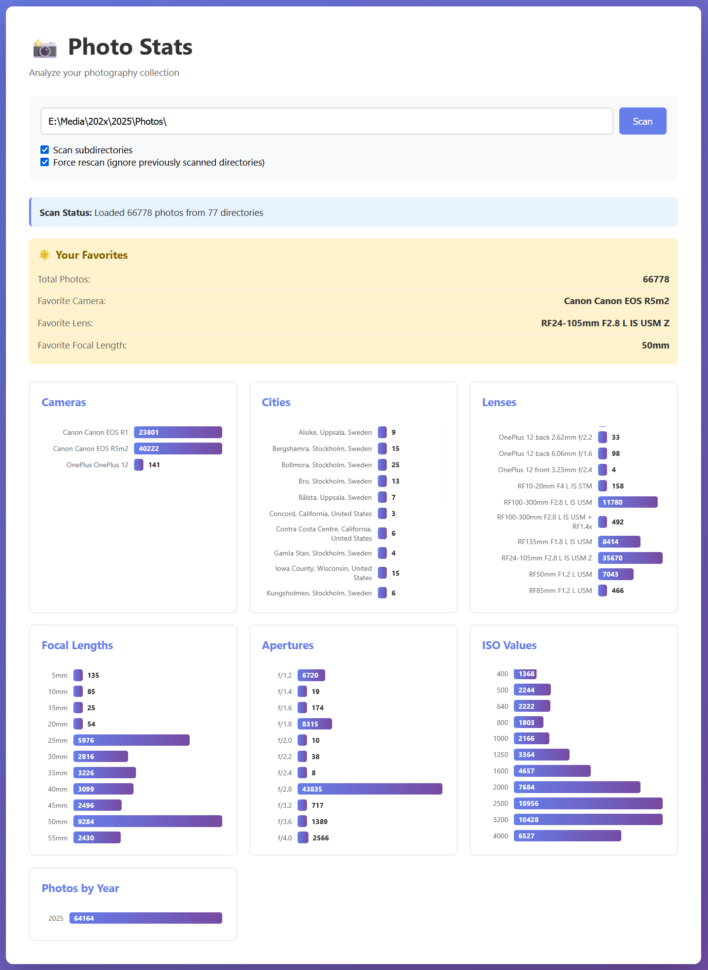
A Python tool for scanning your photo collection and displaying statistics about your photography, such as your favorite lens, focal length, camera, and more. It uses SciPy and a KD-tree to quickly search geolocation data, and display the nearest cities for your photos. The cities data comes from
Countries, States, and Cities database on GitHub.

Photo Stats
WebScan: A product / price / availability scanner
WebScan continuously monitors configured websites, tracks product listings, and alerts you when new products appear. Both email and desktop notifications are supported. It's particularly useful for monitoring e-commerce sites for new inventory, price changes, or specific product availability. You specify the website and a CSS selector for the element to monitor.
